Excel is a convenient software for work,
And hardly restricts the user when typing data.
However, if we consider Excel more than a table for storing data,
There is great importance to the manner of data entry, and especially the data structure.
Proper planning of the structure of the tables will enable analysis and generation of information from the existing data.
A common example is the difference between a flat table and a standard table
(In this article, I will not go into the fundamental differences between them,
Which I explain in great detail in my courses, and I will make do with a demonstration that will present the differences):
Flat table
A flat table is very convenient for entering data.
Suppose we would like to enter the monthly sales of each employee, we will create a flat table (matrix)
And enter the data in the appropriate places (intersection of employee’s name and month):

However, although it is easy to enter data, when we want to analyze them, we encounter difficulty,
First, because the table grows wider, and each time a month is added, we have to correct the formulas,
When transitioning between years, data control becomes even more difficult.
You cannot create a meaningful pivot table from a flat table, Vlookup becomes cumbersome etc.
In fact, a flat table should be the end of the process, not the beginning.
Standard table
A standard table, on the other hand, although more difficult to enter data into, is the beginning of the process, from which the sky is the limit…
What does it look like?
In short, each topic has its own column. If we look at the example above, we seem to have a sales representative, sales month, and amount of sales,
Therefore, a standard table will contain only three columns: representative, month, sales.
Each month we will list the names of their representatives and their sales, in the following format:

It is easy to see that the data input here is more cumbersome, and there is a repetition of the names of the representatives, for each month,
which does not happen in the flat table.
At this point, we understand that a flat table is easy for data entry, but not for analysis,
And we also understand that a standard table is cumbersome to for data entry, but necessary for data extraction
So, what do we do?
Well, it’s good that you ask…
The solution is to enter the data in a flat table, and turn it into a standard table.
How do you do that?
That’s exactly what I’m here for…
First, you need to add the ‘PivotTable and PivotChart Wizard’ to the Quick Access toolbar (for pre-ribbon excel versions).
If you do not have this wizard installed, you can read this article how to add the icon.
Now, we will go through the following steps to create the magic:
- Create a flat table and enter the sales data:
- From the Quick Access Toolbar, click the PivotTable and PivotChart Wizard

- The following window will open, where we’ll select the option ‘Multiple Consolidation Ranges’:

- Click ‘Next‘
- In the second step of the wizard, click ‘Next’ again.

- The following window will open:
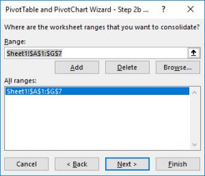
We will select the desired range (note that even if you have previously selected the flat table,
it will not automatically appear in the window)
Click ‘Add‘
We’ll make sure that the range is added to the ‘All Ranges’ window
Click ‘Next’ - In the window that opens, click ‘Finish’.

- And this is where the magic happens – we get the data from the flat table, but this time as a PivotTable!

- Well, here you are sure to ask where is the magic …
I will not leave you in suspense, and I will tell you that all you have to do now
is to double-click on the total amount (in our example, cell H11)
And Excel will create a standard data table from the PivotTable:

- At this point, you can delete column D because it is not needed,
And here we have a standard data table created from the simple entry of a flat table!
Did we already say Magic?